Graphs of Exponential and Logarithmic Functions

Basics of Graphing Exponential Functions

The exponential function

y=b^x

where

b>0

is a function that will remain proportional to its original value when it grows or decays.

Learning Objectives

Describe the properties of graphs of exponential functions

Key Takeaways

Key Points

If the base, $b$ , is greater than $1$ , then the function increases exponentially at a growth rate of $b$ . This is known as exponential growth.
If the base, $b$ , is less than $1$ (but greater than $0$ ) the function decreases exponentially at a rate of $b$ . This is known as exponential decay.
If the base, $b$ , is equal to $1$ , then the function trivially becomes $y=a$ .
The points $(0,1)$ and $(1,b)$ are always on the graph of the function $y=b^x$
The function $y=b^x$ takes on only positive values and has the $x$ -axis as a horizontal asymptote.

Key Terms

exponential growth: The growth in the value of a quantity, in which the rate of growth is proportional to the instantaneous value of the quantity; for example, when the value has doubled, the rate of increase will also have doubled. The rate may be positive or negative. If negative, it is also known as exponential decay.
asymptote: A line that a curve approaches arbitrarily closely. An asymptote may be vertical, oblique or horizontal. Horizontal asymptotes correspond to the value the curve approaches as $x$ gets very large or very small.
exponential function: Any function in which an independent variable is in the form of an exponent; they are the inverse functions of logarithms.

Definitions

At the most basic level, an exponential function is a function in which the variable appears in the exponent. The most basic exponential function is a function of the form

y=b^x

where

b

is a positive number. When

b>1

the function grows in a manner that is proportional to its original value. This is called exponential growth. When

0>b>1

the function decays in a manner that is proportional to its original value. This is called exponential decay.

Graphing an Exponential Function

Example 1

Let us consider the function

y=2^x

when

b>1​

. One way to graph this function is to choose values for

x

and substitute these into the equation to generate values for

y

. Doing so we may obtain the following points:

(-2,\frac{1}{4})[/latex], [latex](-1,\frac{1}{2})[/latex], [latex](0,1)[/latex], [latex](1,2)[/latex] and [latex](2,4)

As you connect the points, you will notice a smooth curve that crosses the

y

-axis at the point

(0,1)

and is increasing as

x

takes on larger and larger values. That is, the curve approaches infinity as

x

approaches infinity. As

x

takes on smaller and smaller values the curve gets closer and closer to the

x

-axis. That is, the curve approaches zero as

x

approaches negative infinity making the

x

-axis is a horizontal asymptote of the function. The point

(1,b)

is on the graph. This is true of the graph of all exponential functions of the form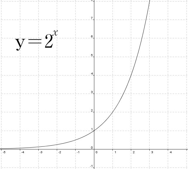

y=b^x

for

x>1

Graph of $y=2^x$ : The graph of this function crosses the

y

-axis at

(0,1)

and increases as

x

approaches infinity. The

x

-axis is a horizontal asymptote of the function.

Example 2

Let us consider the function

y=\frac{1}{2}^x

when

0<b<1

. One way to graph this function is to choose values for

x

and substitute these into the equation to generate values for

y

. Doing so you can obtain the following points:

(-2,4)[/latex], [latex](-1,2)[/latex], [latex](0,1)[/latex], [latex](1,\frac{1}{2})[/latex] and [latex](2,\frac{1}{4})

As you connect the points you will notice a smooth curve that crosses the y-axis at the point

(0,1)

and is decreasing as

x

takes on larger and larger values. The curve approaches infinity zero as approaches infinity. As

x

takes on smaller and smaller values the curve gets closer and closer to the

x

-axis. That is, the curve approaches zero as

x

approaches negative infinity making the

x

-axis a horizontal asymptote of the function. The point

(1,b)

is on the graph. This is true of the graph of all exponential functions of the form

y=b^x

for

0<x<1

. As you can see in the graph below, the graph of

y=\frac{1}{2}^x

is symmetric to that of

y=2^x

over the

y

-axis. That is, if the plane were folded over the

y

-axis, the two curves would lie on each other.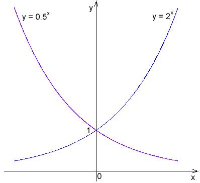

y = 2^x increases from the x axis to infinity. y = .5^x decreases from infinity to the x axis. Both functions are in the positive quadrants (1 and 2) and are symmetric over the y axis.

Graph of $y=2^x$ and $y=\frac{1}{2}^x$ : The graphs of these functions are symmetric over the

y

-axis.

Why Must $b$ Be a Positive Number?

b=1

, then the function becomes

y=1^x

. As

1

to any power yields

1

, the function is equivalent to

y=1

which is a horizontal line, not an exponential equation. If

b

is negative, then raising

b

to an even power results in a positive value for

y

while raising

b

to an odd power results in a negative value for

y

, making it impossible to join the points obtained an any meaningful way and certainly not in a way that generates a curve as those in the examples above.

Properties of Exponential Graphs

The point

(0,1)

is always on the graph of an exponential function of the form

y=b^x

because

b

is positive and any positive number to the zero power yields

1

. The point

(1,b)

is always on the graph of an exponential function of the form

y=b^x

because any positive number

b

raised to the first power yields

1

. The function

y=b^x

takes on only positive values because any positive number

b

will yield only positive values when raised to any power. The function

y=b^x

has the

x

-axis as a horizontal asymptote because the curve will always approach the

x

-axis as

x

approaches either positive or negative infinity, but will never cross the axis as it will never be equal to zero.

Graphs of Logarithmic Functions

Logarithmic functions can be graphed manually or electronically with points generally determined via a calculator or table.

Learning Objectives

Describe the properties of graphs of logarithmic functions

Key Takeaways

Key Points

When graphed, the logarithmic function is similar in shape to the square root function, but with a vertical asymptote as $x$ approaches $0$ from the right.
The point $(1,0)$ is on the graph of all logarithmic functions of the form $y=log{_b}x$ , where $b$ is a positive real number.
The domain of the logarithmic function $y=log{_b}x$ , where $b$ is all positive real numbers, is the set of all positive real numbers, whereas the range of this function is all real numbers.
The graph of a logarithmic function of the form $y=log{_b}x$ can be shifted horizontally and/or vertically by adding a constant to the variable $x$ or to $y$ , respectively.
A logarithmic function of the form $y=log{_b}x$ where $b$ is a positive real number, can be graphed by using a calculator to determine points on the graph or can be graphed without a calculator by using the fact that its inverse is an exponential function.

Key Terms

logarithmic function: Any function in which an independent variable appears in the form of a logarithm. The inverse of a logarithmic function is an exponential function and vice versa.
logarithm: The logarithm of a number is the exponent by which another fixed value, the base, has to be raised to produce that number.
asymptote: A line that a curve approaches arbitrarily closely. Asymptotes can be horizontal, vertical or oblique.

Below are graphs of logarithmic functions with bases 2,

e

, and 10.

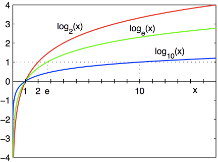Logarithmic Graphs: After

x=1

, where the graphs cross the

x

-axis,

\log_2(x)

in red is above

\log_e(x)

in green, which is above

\log_{10}(x)

in blue. Before this point, the order is reversed. All three logarithms have the

y

-axis as a vertical asymptote, and are always increasing.

All three logarithmic graphs begin with a steep climb after

x=0

, but stretch more and more horizontally, their slope ever-decreasing as

x

increases. All of them cross the

x

-axis at

x=1

Properties of the Graphs of Logarithmic Functions

Special Points

The graph crosses the

x

-axis at

1

. That is, the graph has an

x

-intercept of

1

, and as such, the point

(1,0)

is on the graph. In fact, the point

(1,0)

will always be on the graph of a function of the form

y=log{_b}x

where

b>0

. This is because for

x=1

, the equation of the graph becomes

y=log{_b}1

. Thus, we are looking for an exponent

y

such that

b^y=1

. As

b>0

, the exponent we seek is

1

irrespective of the value of

b

. This means the point

(x,y)=(1,0)

will always be on a logarithmic function of this type.

Asymptotes

The

y

-axis is a vertical asymptote of the graph. This means that the curve gets closer and closer to the

y

-axis but does not cross it. Let us consider what happens as the value of

x

approaches zero from the right for the equation whose graph appears above. Namely,

y=log{_b}x

. We can do this by choosing values for

x

, plugging them into the equation and generating values for

y

. Let us assume that

b

is a positive number greater than

1

, and let us investigate values of

x

between

0

and

1

. Under these conditions, if we let

x=\frac{1}{b}

, the equation becomes

y=log\frac{1}{b}

. Thus, we are looking for an exponent such that

b

raised to that exponent yields

\frac{1}{b}

. The exponent we seek is

-1

and the point

(\frac{1}{b},-1)

is on the graph. Similarly, we can obtain the following points that are also on the graph:

(\frac{1}{b^2},-2),(\frac{1}{b^3},-3),(\frac{1}{b^4},-4)

and so on If we take values of

x

that are even closer to

0

, we can arrive at the following points:

(\frac{1}{b^{10}},-10),(\frac{1}{b^{100}},-100)

and

(\frac{1}{b^{1000}},-1000)

As can be seen the closer the value of

x

gets to

0

, the more and more negative the graph becomes. That is, as

x

approaches zero the graph approaches negative infinity. This means that the

y

-axis is a vertical asymptote of the function.

Domain and Range

The domain of the function is all positive numbers. That means that the

x

-value of the function will always be positive. Let us begin by considering why the

x

-value of the curve is never

0

. If the

x

-value were zero, the function would read

y=log{_b}0

. Here we are looking for an exponent such that

b

raised to that exponent is

0

. Since

b

is a positive number, there is no exponent that we can raise

b

to so as to obtain

0

. In fact, since

b

is positive, raising it to a power will always yield a positive number. The range of the function is all real numbers. That is, the graph can take on any real number.

Comparing $y=log{_x}$ and $y=\sqrt{x}$

At first glance, the graph of the logarithmic function can easily be mistaken for that of the square root function.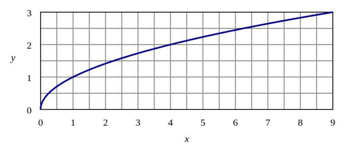

Half of a sideways parabola (u-shaped curve) with a vertex at the origin. It does not have a vertical asymptote like a logarithmic function, as it touches the y-axis.

Graph of $y=\sqrt{x}$ : The graph of the square root function resembles the graph of the logarithmic function, but does not have a vertical asymptote.

Both the square root and logarithmic functions have a domain limited to

x

-values greater than

0

. However, the logarithmic function has a vertical asymptote descending towards

-\infty

x

approaches

0

, whereas the square root reaches a minimum

y

-value of

0

. The range of the square root function is all non-negative real numbers, whereas the range of the logarithmic function is all real numbers.

Graphing Logarithmic Functions

Graphing logarithmic functions can be done by locating points on the curve either manually or with a calculator. When graphing without a calculator, we use the fact that the inverse of a logarithmic function is an exponential function. When graphing with a calculator, we use the fact that the calculator can compute only common logarithms (base is

10

), natural logarithms (base is

e

) or binary logarithms (base is

2

). Of course, if we have a graphing calculator, the calculator can graph the function without the need for us to find points on the graph.

Graphing Logarithmic Functions Using Their Inverses

Logarithmic functions can be graphed by hand without the use of a calculator if we use the fact that they are inverses of exponential functions. Let us again consider the graph of the following function:

y=log{_3}x

This can be written in exponential form as:

3^y=x

Now let us consider the inverse of this function. To do so, we interchange

x

and

y

3^x=y

The exponential function

3^x=y

is one we can easily generate points for. If we take some values for

x

and plug them into the equation to find the corresponding values for

y

we can obtain the following points:

(-2,\frac{1}{9}),(-1,\frac{1}{3}),(0,1),(1,3),(2,9)[/latex] and [latex](3,27)

Now we must note that these points are not on the original function (

y=log{_3}x

) but rather on its inverse

3^x=y

. However, if we interchange the

x

and

y

-coordinates of each point we will in fact obtain a list of points on the original function. These are:

(\frac{1}{9},-2),(\frac{1}{3},-1),(1,0),(3,1),(9,2)

and

(27,3)

. We plot and connect these points to obtain the graph of the function

y=log{_3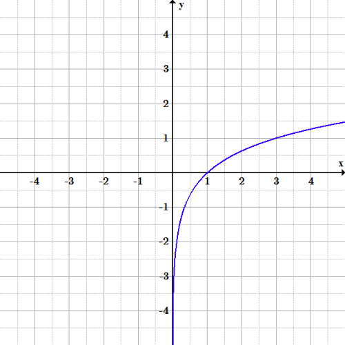}x

below.

Graph of $y=log{_3}x$ : The graph of the logarithmic function with base

3

can be generated using the function's inverse. Its shape is the same as other logarithmic functions, just with a different scale.

Graphing Logarithmic Functions With Bases Between $0$ and $1$

Thus far we have graphed logarithmic functions whose bases are greater than

1

. If we instead consider logarithmic functions with a base

b

, such that

0<b<1

, we get a graph that is very similar to those we have seen already. In fact if

b>0

, the graph of

y=log{_b}x

and the graph of

y=log{_\frac{1}{b}}x

are symmetric over the

x

-axis. Thus, if we identify a point

(x,y)

on the graph of

y=log{_b}x

, we can find the corresponding point on

y=log{_\frac{1}{b}}x

by changing the sign of the

y

-coordinate. The corresponding point is

(x,-y)

. Here is an example for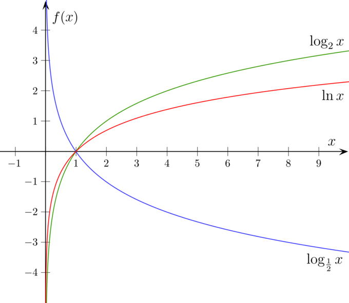

b=2

log_2(x) is increasing from the y-axis (its vertical asymptote) to infinity. log_.5(x) is decreasing from the y-axis (also its vertical asymptote) to negative infinity.

Graphs of $log{_2}x$ and $log{_\frac{1}{2}}x$ : The graphs of

log_2 x

and

log{_\frac{1}{2}}x

are symmetric over the x-axis

Solving Problems with Logarithmic Graphs

Some functions with rapidly changing shape are best plotted on a scale that increases exponentially, such as a logarithmic graph.

Learning Objectives

Convert problems to logarithmic scales and discuss the advantages of doing so

Key Takeaways

Key Points

Logarithmic graphs use logarithmic scales, in which the values differ exponentially. For example, instead of including marks at $0,1,2$ and $3$ , a logarithmic scale may include marks at $0.1, 1, 10$ and $100$ , each an equal distance from the previous and next.
Logarithmic graphs allow one to plot a very large range of data without losing the shape of the graph.
Logarithmic graphs make it easier to interpolate in areas that may be difficult to read on linear axes. For example, if the plot $y=x^5$ is scaled to show a very wide range of $y$ values, the curvature near the origin may be indistinguishable on linear axes. It is much clearer on logarithmic axes.

Key Terms

logarithm: The logarithm of a number is the exponent by which another fixed value, the base, has to be raised to produce that number.
interpolate: To estimate the value of a function between two points between which it is tabulated.

Why Use a Logarithmic Scale?

Many mathematical and physical relationships are functionally dependent on high-order variables. This means that for small changes in the independent variable there are very large changes in the dependent variable. Thus, it becomes difficult to graph such functions on the standard axis. Consider, as an example, the Stefan-Boltzmann law, which relates the power (j^*) emitted by a black body to temperature (T).

j^*= \sigma T^4

On a standard graph, this equation can be quite unwieldy. The fourth-degree dependence on temperature means that power increases extremely quickly. The fact that the rate is ever-increasing (and steeply so) means that changing scale (scaling the axes by

5

10

or even

100

) is of little help in making the graph easier to interpret. For very steep functions, it is possible to plot points more smoothly while retaining the integrity of the data: one can use a graph with a logarithmic scale, where instead of each space on a graph representing a constant increase, it represents an exponential increase. Where a normal (linear) graph might have equal intervals going 1, 2, 3, 4, a logarithmic scale would have those same equal intervals represent 1, 10, 100, 1000. Here are some examples of functions graphed on a linear scale, semi-log and logarithmic scales. The top left is a linear scale. The bottom right is a logarithmic scale. The top right and bottom left are called semi-log scales because one axis is scaled linearly while the other is scaled using logarithms.

The linear and logarithmic scales preserve the relative shapes of the functions. The semi-log scales, where only the x or y axis is on a logarithmic scale, skew the shapes of the graphs relative to both axes having the same scale.

Logarithmic scale: The graphs of functions

f(x)=10^x,f(x)=x

and

f(x)=\log x

on four different coordinate plots. Top Left is a linear scale, top right and bottom left are semi-log scales and bottom right is a logarithmic scale.

As you can see, when both axis used a logarithmic scale (bottom right) the graph retained the properties of the original graph (top left) where both axis were scaled using a linear scale. That means that if we want to graph a function that is unwieldy on a linear scale we can use a logarithmic scale on each axis and retain the properties of the graph while at the same time making it easier to graph.

With the semi-log scales, the functions have shapes that are skewed relative to the original. When only the

x

-axis has a log scale, the logarithmic curve appears as a line and the linear and exponential curves both look exponential. When only the

y

-axis has a log scale, the exponential curve appears as a line and the linear and logarithmic curves both appear logarithmic.It should be noted that the examples in the graphs were meant to illustrate a point and that the functions graphed were not necessarily unwieldy on a linearly scales set of axes.

Converting Linear to Logarithmic Scales

The primary difference between the logarithmic and linear scales is that, while the difference in value between linear points of equal distance remains constant (that is, if the space from

0

1

on the scale is

1

cm on the page, the distance from

1

2

2

3

, etc., will be the same), the difference in value between points on a logarithmic scale will change exponentially. A logarithmic scale will start at a certain power of

10

, and with every unit will increase by a power of

10

. Thus, if one wanted to convert a linear scale (with values

0-5

to a logarithmic scale, one option would be to replace

1,2,3,4

and 5 with

0.001,0.01,0.1,1,10

and

100

, respectively. Between each major value on the logarithmic scale, the hashmarks become increasingly closer together with increasing value. For example, in the space between

1

and

10

, the

8

and

9

are much closer together than the

2

and

3

. The advantages of using a logarithmic scale are twofold. Firstly, doing so allows one to plot a very large range of data without losing the shape of the graph. Secondly, it allows one to interpolate at any point on the plot, regardless of the range of the graph. Similar data plotted on a linear scale is less clear.

Solving Problems Using Logarithmic Graphs

A key point about using logarithmic graphs to solve problems is that they expand scales to the point at which large ranges of data make more sense. In the equation mentioned above (

j^*= \sigma T^4

), plotting

j

vs.

T

would generate the expected curve, but the scale would be such that minute changes go unnoticed and the large scale effects of the relationship dominate the graph: It is so big that the "interesting areas" won't fit on the paper on a readable scale. Taking the logarithm of each side of the equations yields:

logj=log{(\sigma\tau ) }^4

. We now rely on the properties of logarithms to re-write the equation. Recall the following properties of logarithms:

\log(ab)=\log(a)+\log(b) \\ \log(a)^b=(b)\log(a)

Using the above, our equation becomes:

\begin{align} \log j&=4\log{(\sigma\tau ) } \\ &=4\log{(\sigma)}+4\log{(\tau ) } \\ &=4\log{(\tau ) }+4\log{(\sigma)} \end{align}

Graphs of Exponential and Logarithmic Functions

Basics of Graphing Exponential Functions

Learning Objectives

Key Takeaways

Key Points

Key Terms

Definitions

Graphing an Exponential Function

Example 1

Example 2

Why Must $b$ Be a Positive Number?

Properties of Exponential Graphs

Graphs of Logarithmic Functions

Learning Objectives

Key Takeaways

Key Points

Key Terms

Properties of the Graphs of Logarithmic Functions

Special Points

Asymptotes

Domain and Range

Comparing $y=log{_x}$ and $y=\sqrt{x}$

Graphing Logarithmic Functions

Graphing Logarithmic Functions Using Their Inverses

Graphing Logarithmic Functions With Bases Between $0$ and $1$

Solving Problems with Logarithmic Graphs

Learning Objectives

Key Takeaways

Key Points

Key Terms

Why Use a Logarithmic Scale?

Converting Linear to Logarithmic Scales

Solving Problems Using Logarithmic Graphs

Licenses & Attributions

CC licensed content, Shared previously

CC licensed content, Specific attribution

Study Guides > Boundless Algebra

Graphs of Exponential and Logarithmic Functions

Basics of Graphing Exponential Functions

Learning Objectives

Key Takeaways

Key Points

Key Terms

Definitions

Graphing an Exponential Function

Example 1

Example 2

Why Must bbb Be a Positive Number?

Properties of Exponential Graphs

Graphs of Logarithmic Functions

Learning Objectives

Key Takeaways

Key Points

Key Terms

Properties of the Graphs of Logarithmic Functions

Special Points

Asymptotes

Domain and Range

Comparing y=logxy=log{_x}y=logx​ and y=xy=\sqrt{x}y=x​

Graphing Logarithmic Functions

Graphing Logarithmic Functions Using Their Inverses

Graphing Logarithmic Functions With Bases Between 000 and 111

Solving Problems with Logarithmic Graphs

Learning Objectives

Key Takeaways

Key Points

Key Terms

Why Use a Logarithmic Scale?

Converting Linear to Logarithmic Scales

Solving Problems Using Logarithmic Graphs

Licenses & Attributions

CC licensed content, Shared previously

CC licensed content, Specific attribution

Why Must $b$ Be a Positive Number?

Comparing $y=log{_x}$ and $y=\sqrt{x}$

Graphing Logarithmic Functions With Bases Between $0$ and $1$